Chasing Significance: Are you p-hacking in your research?

What is p-hacking

P-hacking, also known as data fishing or data dredging, is a serious problem in research that undermines the credibility and reliability of findings by increasing the likelihood of false positives and leading to misleading conclusions. It is a form of statistical bias where data or analysis is manipulated to artificially produce statistically significant results. You might have fallen into the trap of p-hacking without even realizing it—perhaps influenced by the way you were taught statistics. This analysis will demonstrate how p-hacking can lead to spurious findings and illustrate the risks of data exploration without proper safeguards.

Does Listening to Music Affect Study Time?

Dr. Ch. Picking is interested in understanding how music affects study habits. He conducted a survey of 600 university students, collecting data on two variables:

- Whether they listen to music while studying

- How many hours they study per day

Let's simulate the data for this study. We will generate two independent variables. The first variable, `study_hours`, represents the number of hours a student studies per day. We will assume that this variable follows a normal distribution with a mean of 3 hours and a standard deviation of 1 hour. The second variable, `listening`, represents whether a student listens to music while studying. We will assume that 45% of students listen to music while studying.

# Initial Data Generation 
set.seed(42)
students = 600
p_listen_music = 0.45

# Draw initial sample
study_hours = rnorm(students, mean = 3, sd = 1)  # Study hours normally distributed around 3
listening = sample(c('music', 'no music'), students, replace = TRUE,
                  prob = c(p_listen_music, 1 - p_listen_music))

# Create initial dataframe
data = data.frame('study_hours' = study_hours, 'listening' = listening)
head(data)

  study_hours listening
1    4.370958  no music
2    2.435302  no music
3    3.363128     music
4    3.632863  no music
5    3.404268     music
6    2.893875     music

First, let's visualize the distribution of study hours between music listeners and non-listeners:

# Visualization of initial data
library(ggplot2)
options(repr.plot.width = 5, repr.plot.height = 4)

# Boxplot for music listening vs study hours
ggplot(data) +
  geom_boxplot(aes(x = listening, y = study_hours, fill = listening), alpha = 0.5, outlier.shape = NA) + # Boxplots, remove outliers
  geom_jitter(aes(x = listening, y = study_hours), width = 0.2, height = 0, size = 1, alpha = 0.3) + # Jittered points
  scale_fill_manual(breaks = c('music', 'no music'), values = c('purple', 'white')) +
  theme(legend.position = "none", plot.title = element_text(hjust = 0.5)) +
  xlab('Listening to Music') +
  ylab('Study Hours') +
  ggtitle('Distribution of Study Hours 
for Students With/Without Music')

Let’s conduct a formal statistical test, specifically a two-sample t-test. The null hypothesis is “Listening to music while studying does not affect the number of hours students study per day”.

# Initial t-test
t.test(study_hours ~ listening, data = data)

	Welch Two Sample t-test

data:  study_hours by listening
t = 0.061927, df = 583.39, p-value = 0.9506
alternative hypothesis: true difference in means between group music and group no music is not equal to 0
95 percent confidence interval:
 -0.1532923  0.1632737
sample estimates:
   mean in group music mean in group no music 
              2.978125               2.973135 

The resulting p-value is high, i.e. p = 0.9506>0.05, so we cannot reject the null. In other words, we conclude that there is not enough evidence to say that listening to music is associated with study time. (Actually, we are not surprised as the two variables were generated independently of each other).

Disappointed by their non-significant p-value and worried that these results might not be accepted for publication, Dr. Ch. Picking and colleagues explored an alternative hypothesis: "What if different types of music have different effects? Maybe classical music helps while heavy metal distracts?". This seems like a reasonable question. After all, different genres of music might have different effects on concentration.

Exploring the effect of music genre

Let's break down the analysis by music genre:

# Adding Genre Analysis
library(tidyverse)
set.seed(42)

# Create list of music genres
genres = c('classical', 'jazz', 'world', 'pop', 'electronic', 'ambient',
           'hip-hop', 'rock', 'folk', 'blues', 'reggae', 'country',
           'latin', 'indie', 'r&b', 'trap', 'instrumental', 'techno', 
           'metal', 'punk')

# Add genre column to the data
data$music_genre = sample(genres, students, replace = TRUE)
data = data %>%
  mutate(music_genre = ifelse(listening == "no music", NA, music_genre))

# Create a custom color palette for visualization
custom_colors = c(
    "#1f77b4", "#ff7f0e", "#2ca02c", "#d62728", "#9467bd",  
    "#8c564b", "#e377c2", "#7f7f7f", "#bcbd22", "#17becf",  
    "#aec7e8", "#ffbb78", "#98df8a", "#ff9896", "#c5b0d5",  
    "#c49c94", "#f7b6d2", "#c7c7c7", "#dbdb8d", "#9edae5"   
)

Let's visualize study hours across different genres:

ggplot(data %>% filter(!is.na(music_genre))) +
  geom_boxplot(aes(x = music_genre, y = study_hours, fill = music_genre), alpha = 0.5, outlier.shape = NA) +  # Boxplots with alpha for transparency, remove outliers
  geom_jitter(aes(x = music_genre, y = study_hours), width = 0.2, height = 0, size = 1, alpha = 0.3) + # Jittered points
  scale_fill_manual(values = custom_colors) +
  xlab('Music Genre') +
  ylab('Study Hours') +
  theme_minimal() +
  theme(
    legend.position = "none",
    axis.text.x = element_text(angle = 45, hjust = 1),
    panel.grid.major.x = element_blank(),
    plot.title = element_text(hjust = 0.5)
  ) +
  ggtitle("Study Hours Distribution by Music Genre")

Let's test each genre individually:

# Function to test specific genre
test_genre = function(genre) {
  data = data %>%
    mutate(listening_genre = ifelse(music_genre != genre |
                                  is.na(music_genre), "no", "yes"))
  t.test(study_hours ~ listening_genre, data = data)$p.value
}

# Testing some of the individual genres
cat('p value for classical = ', test_genre('classical'), '
')
cat('p value for trap = ', test_genre('trap'), '
')
cat('p value for rock = ', test_genre('rock'), '
')
cat('p value for metal = ', test_genre('metal'), '
')

p value for classical =  0.9662414 
p value for trap =  0.02818423 <- Eureka!
p value for rock =  0.9481007 
p value for metal =  0.6340543 

Oh, here’s a statistically significant result for trap music! Let's visualize all p-values:

# Visualization of p-values for all genres
ttest_data = data.frame('genre' = genres,
                       'pval' = sapply(genres, test_genre))

ggplot(ttest_data) +
    geom_point(aes(x = genre, y = pval, color = genre), size = 5) +
    scale_color_manual(values = custom_colors) +
    geom_hline(aes(yintercept = 0.05), linetype = 'dashed') +
    ylim(0, 1) +
    xlab('Music Genre') +
    ylab('p-value') +
    theme_minimal() +
    theme(
        legend.position = "none",
        axis.text.x = element_text(angle = 45, hjust = 1),
        panel.grid.major.x = element_blank(),
        plot.title = element_text(hjust = 0.5)
    ) +
    ggtitle("P-values by Music Genre: Identifying Significant Results")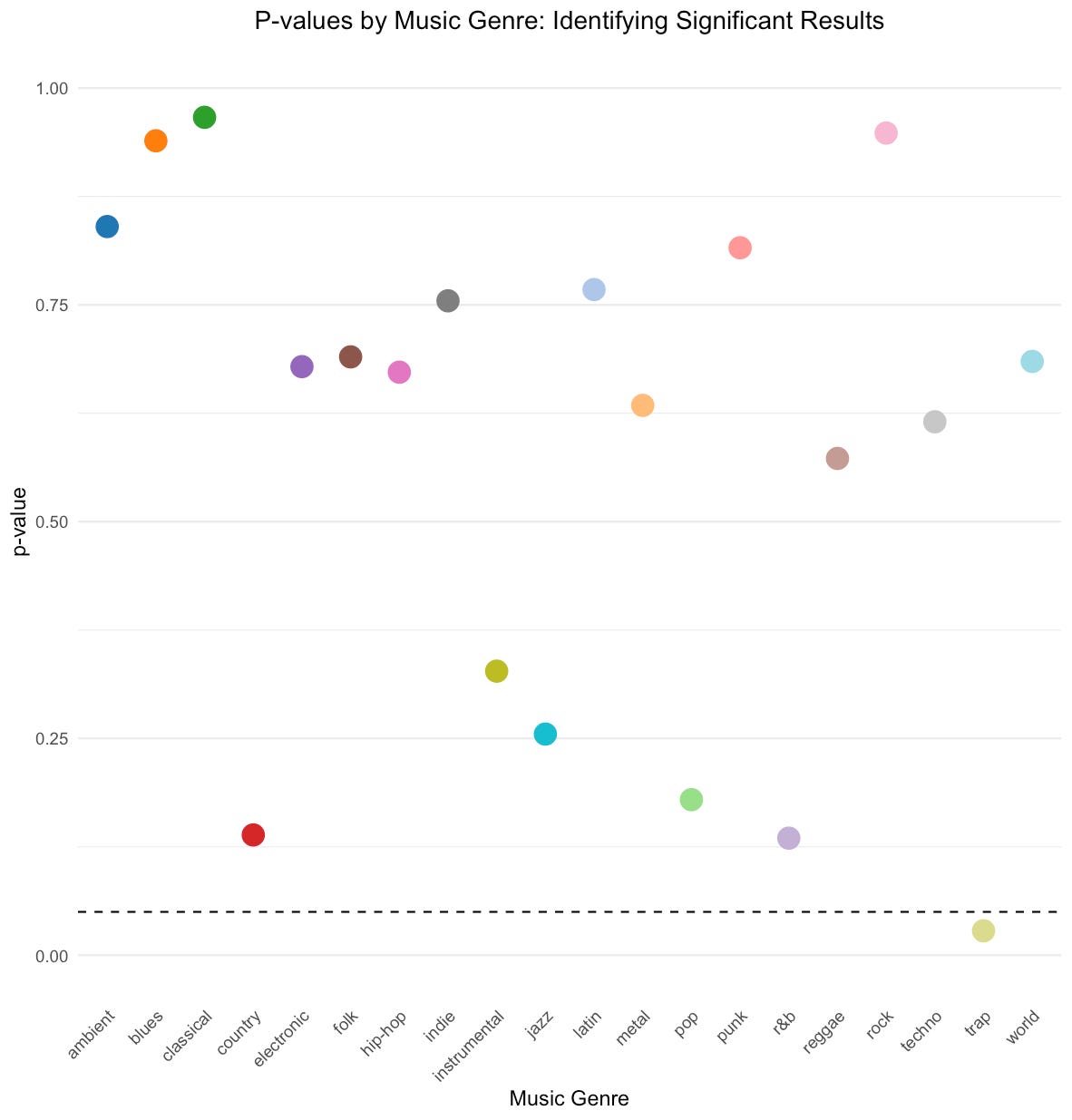

Can you see this dot under the dashed line? It represents the p-value corresponding to trap music (p = 0.028).

The Multiple Testing Trap

Exciting news! The study findings reveal that students who listen to trap music tend to study less. Dr. Ch. Picking and colleagues have started exploring relevant literature to support this finding, are preparing a preprint for publication, and have even given an interview to a news website to discuss their (unpublished) work.

News Headlines:

- "Trap Music: The Soundtrack to Procrastination?"

- "Beats or Books? Trap Music Tied to Fewer Study Hours"

- "Trapped in the Beat: How Trap Music May Be Cutting Study Time"

- "Drop the Bass, Pick Up the Books: Trap Music Linked to Reduced Study Habits"

But wait... is this result trustworthy? Let's understand what's happening here.

Even if there is no real effect of listening to music on study time, the probability of observing a statistically significant result remains 0.05. This is known as the Type I error rate. This happens because, under the null hypothesis, p-values are uniformly distributed, meaning the likelihood of observing a p-value less than 0.05 is exactly 5%.

While the formal proof of this fact is straightforward, it can also be verified through simulation. To do this, we can generate data for study time and music listening 10,000 times, perform a t-test on each dataset to test the null hypothesis ("there is no effect of listening to music on study time"), and examine the resulting distribution of p-values.

# Function to generate data
generate_data = function() {
  study_hours = rnorm(students, mean = 3, sd = 1)
  listening = sample(c('music', 'no music'), students, replace = TRUE,
                    prob = c(p_listen_music, 1 - p_listen_music))
  data = data.frame('study_hours' = study_hours, 'listening' = listening)
  return(data)
}

# Compute p-values for 10000 random data sets
trial = 10000
pvals = replicate(trial,
                 t.test(study_hours ~ listening,
                        data = generate_data())$p.value)

# Visualization of p-value distribution
ggplot() +
  geom_histogram(aes(x = pvals, y = after_stat(density)), # Corrected line
                 breaks = seq(0, 1, 0.1),
                 fill = 'purple',
                 alpha = 0.5) +
  ggtitle("Distribution of p-values under null hypothesis") +
  xlab("p-value") +
  ylab("Density")

Therefore, if we conduct multiple analyses on these random datasets (as we did with different music genres), we would expect some p-values to fall below the standard significance threshold (typically 0.05) purely by chance. This highlights the risks of conducting numerous tests without proper adjustments for multiple comparisons.

What Have We Learned?

This investigation demonstrates a classic case of p-hacking. Here's what happened:

1. Dr Ch. Picking et al. started with a simple question about music and study time

2. Finding no significant results, they divided their analysis into 20 different genres

3. By testing 20 different hypotheses, they increased their chances of finding a "significant" result by chance

4. With 20 tests and a significance level of 0.05, they had a

\((1-0.95^{20}) \times 100 = 64.14\%\)

chance of finding at least one "significant" result by chance, that is even if no real relationship exists!

Recommendations for Avoiding p-hacking

1. Pre-register your hypotheses: Decide which hypothesis you want to test before looking at the data

2. Use multiple testing corrections: When testing multiple hypotheses, adjust your significance levels (e.g., Bonferroni correction, Benjamini and Hochberg's false discovery rate). For instance, using Bonferroni correction with 20 tests, adjust α from 0.05 to 0.05/20 = 0.0025.

3. Validate on fresh data: If possible, collect new data to test any relationships discovered through exploration or use cross-validation to validate your hypothesis

4. Report all tests: Document all analyses performed, not just the significant ones

Remember: The more you look, the more likely you are to find something - even if it's not really there!